Coordicide Update — Autopeering: Part 1
The Autopeering Module
A few months ago, we opened up the source code of GoShimmer, IOTA’s prototype and research tool to experiment and test the building blocks of Coordicide. We are thrilled to see such a big and productive engagement from the community and we want to thank you all for your contributions and feedback! They have been very useful to improve GoShimmer as well as to help us identify how to better redesign the autopeering module.
We are excited to share with you the source code of the improved redesign of the autopeering module. You can access the code from the following repository:
https://github.com/iotaledger/autopeering-sim
In the IOTA protocol, a node (or peer) is a machine storing the information about the Tangle, IOTA’s underlying data structure. Nodes also commonly act as the entry point for accessing and utilizing the Tangle. In order for the network to work efficiently, nodes exchange information with each other to be kept up-to-date about the new ledger state. Currently, a manual peering or connection process is used for nodes to register mutually as neighbors. However, manual peering might be subject to attacks (e.g., social engineering) to affect the network topology. To prevent these attacks, and to simplify the setup process of new nodes, we introduced, in the Coordicide white paper, a mechanism that allows nodes to choose their neighbors automatically. The process of nodes choosing their neighbors without manual intervention by the node operator is called autopeering.
The aim of the autopeering module redesign is to ease simulations while keeping the same code base that will be used in GoShimmer. Being able to assess the autopeering behavior and performance via simulations is very important for IOTA. It allows answering several questions, such as how many peering requests each node has to send on average before getting accepted, how long a connection is going to last, how fast the protocol converges, and so on. Moreover, it sets the ground for studying attack vectors in a controlled environment.
We have logically divided the autopeering module into two main submodules: peer discovery and neighbor selection. The former is responsible for operations, such as discovering new peers and verifying their online status. The latter is responsible for finding and managing neighbors for IOTA’s nodes. We have also encapsulated the network layer (P2P communication) and the storage layer (persisting peer information) through the use of Go interfaces. You can see a high-level overview of the design in the following figure:

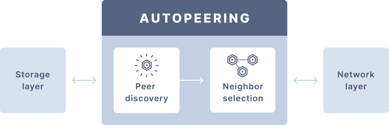
With this design, it is easily possible to switch from a database to a much more lightweight in-memory storage and to switch from connections between servers to inter-process communication. Servers and a database are required for GoShimmer. Replacing them makes writing an efficient simulation running on a single computer as easy as writing just a few lines of code.
As a demonstrator, we have written a simulation that focuses on the neighbor selection submodule. In the simulation, we assume that the peer discovery knows all the nodes in the network to be able to evaluate solely the effect of the peer selection. Scenarios with a partial view of the network as well as the performance of the peer discovery will be the subject of further simulations and analysis.
The neighbor selection and, in particular, the decision about which potential neighbors are preferable, are made on the basis of their distance. This distance function is based on the private and public salts, as defined in the Coordicide white paper. As a next step, we will add Mana-depending distances.
Currently, the simulation can be configured with the following parameters:
- N: the total number of peers
- T: the salt lifetime, in seconds
- SimDuration: the duration of the simulation, in seconds
- VisualEnabled: the toggle to enable/disable the simulation visualizer, accessible at http://localhost:8844 after starting the simulation
- dropAll: the toggle to enable/disable dropping all the neighbors at each salt update
The following animation has been recorded while running the simulation with the visualizer enabled. It provides us with a nice visual representation of the peering process:
Newly established links between peers are highlighted in blue, with the requesting and the accepting peer shown in blue and green respectively. Dropped links are highlighted in red.
Currently, the simulator supports the following metrics for which we provide evaluation scripts:
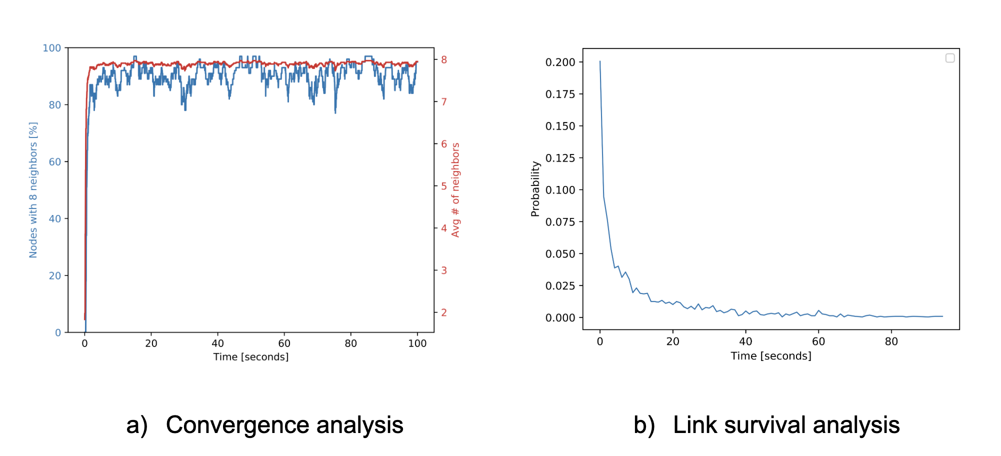
- Convergence: the proportion of peers that have the maximum number of neighbors
- Link survival time: the probability that a given link is still active after a certain amount of time
- Message analysis: statistics about the number of messages sent and received (peering requests, peering responses, and connection drops)
We also include an evaluation script, plot.py, written in Python with Matplotlib. This script extracts the data from CSV-output files, that are produced by the simulation code, and generates plots for both the convergence and the link survival time.
For example, from the figures below, you can see: a) the percentage of nodes with 8 neighbors (in this configuration 8 is the maximum number of neighbors) and the average number of neighbors over time and b)the probability that a given link would last a certain amount of time.
Moreover, running the simulation produces a CSV file (inside the data folder) with the data of the message analysis. You can see an example of that in the following table:
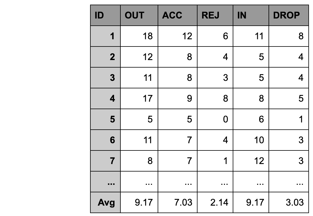
Here, the average number of peering requests sent (OUT going) is equal to the average number of peering requests received (IN coming). It is easy to calculate the average number of peering requests sent before gettingACCepted: by just dividing the outgoing requests over the accepted requests. That is, in this example, 9.17 / 7.03 = 1.3. We can also extract information about the rate at which connections get DROP ped: in this example, one peer gets replaced on average for every 9.17 / 3.03 = 3.02 incoming messages.
We will continue to develop more simulations for the peer discovery and the neighbor selection, and add them to the repository! We also have the goal to eventually port the code from the simulations into GoShimmer. Thanks to the flexibility and modularity of the autopeering and GoShimmer, this will be possible with only a few adaptations. If that challenge sounds interesting, you are more than welcome to help IOTA with the integration! Furthermore, we are evaluating the possibility of an integration of the autopeering into the current IOTA protocol (with the Coordinator) as part of a series of improvements for the official mainnet.
In the next part of the autopeering blog post series, we will dive deeper into the inner workings of this module. In the meantime, we hope this code can be useful for anyone interested in analyzing the autopeering module. You are invited to contribute to the code with new features! Alternatively, you can run the simulation and provide feedback or you can check out our open call for the Coordicide grant program to find out about further collaboration opportunities.
As always, we welcome your comments and questions either here or on IOTA’s official Discord server, in the#tanglemath or #goshimmer-discussion channel.
Follow us on our official channels for the latest updates
Discord | Twitter | LinkedIn | Instagram | YouTube