Running on the Tangle: a Marathon of Random Walkers

In today’s blog post, we’ll have a closer look at the journey of random walkers. Similar to one of our previous posts on mixing time in the Tangle, we are interested in understanding how long random walkers have to walk to select a tip and, more importantly, how long they take to reach their goal. For this analysis, we will simulate different Tangles and, for each one, we will release 100,000 random walkers starting from the Genesis and measure their velocity while performing a random walk on the Tangle. This article assumes a basic understanding of how the Tangle is built and probability theory, as we will touch on topics such as the parameter α, direct approvers, and probability density functions(PDF). If you are not familiar with these topics, we suggest you read up on them first.

We can start by defining what exactly we mean by velocity. Consider a Tangle with N transactions. To each transaction, we assign an ID according to the time of announcement to the network i.e., the Genesis transaction has ID 1, the first transaction that approves the genesis has ID 2, and so on. We can assume that those transactions are announced to the network at times t_1 < t_2 < … < t_N. We define the following quantities:

distance(x-y)= ID_y - ID_x
velocity(x-y)=distance(x-y) / steps

Basically, we define the distance between two transactions x and y as the number of transactions announced to the network within the interval that goes from t_x to t_y. Similarly, we define the velocity of a random walker transitioning from a transaction x to a transaction y as the distance covered by the walker divided by the total number of steps required to complete that transition.

Now, to give you a graphical representation of these concepts, we can have a look at this example:

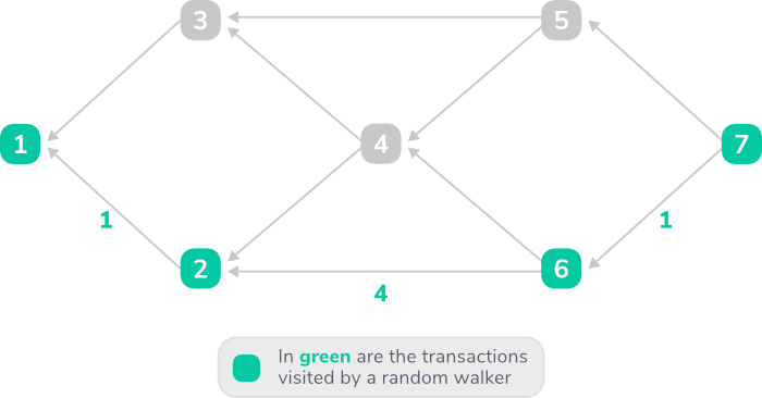
First, we recall that a random walker walks from the past to the present, thus it traverses the Tangle in opposite directions with respect to the direction of the links. Here, our random walker starts from transaction 1, and then transitions to transaction 2. During this transition, the distance covered is obtained by subtracting the ID of the current transaction (2) from the ID of the starting transaction (1), so the result is 2 -1 = 1. Following its next steps, we can see that during the transition from transactions 2 to 6, and from transactions 6 to 7, the random walker covers a distance of4and1respectively. Thus, the velocity of our random walker is on average2transactions per step.

Here is another example.

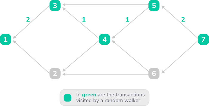
Here, as the previous example, our random walker starts its journey from the transaction with ID 1 and reaches the tip with ID 7. But this time, the random walker chooses a different path. It traverses the Tangle by walking over transactions 1, 3, 4, 5 and 7, covering a distance of6transactions over 4 steps, and thus has an average velocity of1.5transactions per step.

Now, having clear what we mean by velocity, we can ask the following question:what is the probability for a random walker to experience a given velocity?Intuitively, both distance and velocity depend on which direct approver a random walker selects to perform its next transition. More specifically, we consider a transactionx. We can sort its direct approvers based on their arrival time as 1-st, 2-nd, 3-rd, …, and last approver, just like in this example:

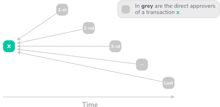
Since the 1-st approver has a smaller ID with respect to the ID of the last approver (i.e., the first approver has been announced to the network before the last approver), values of both distance covered and velocity of our random walker transitioning from x to the first approver will be smaller than if transitioning from x to the last approver.

We can confirm this intuition by running some simulations. For simplicity, we consider a Tangle built according to the uniform random tip selection(URTS) with an arrival rate λ = 100. Once our Tangle reaches a size of 100,000 transactions, we unleash 100,000 random walkers starting from the Genesis and we measure their velocity for the following variants:

while performing an unbiased random walk (URW, i.e., a random walk with parameter α=0);
while performing a walk transitioning always to the first direct approver (lower bound of velocity);
while performing a walk transitioning always to the last direct approver, if, more than one direct approver exists (i.e., we discard transactions that only have one approver, otherwise would be as transitioning to the first approver)(upper bound of velocity);

For all the transactions, we also measure the distance between each transaction and its direct approvers. We then plot the probability density function(PDF) that you can see in the following figure.

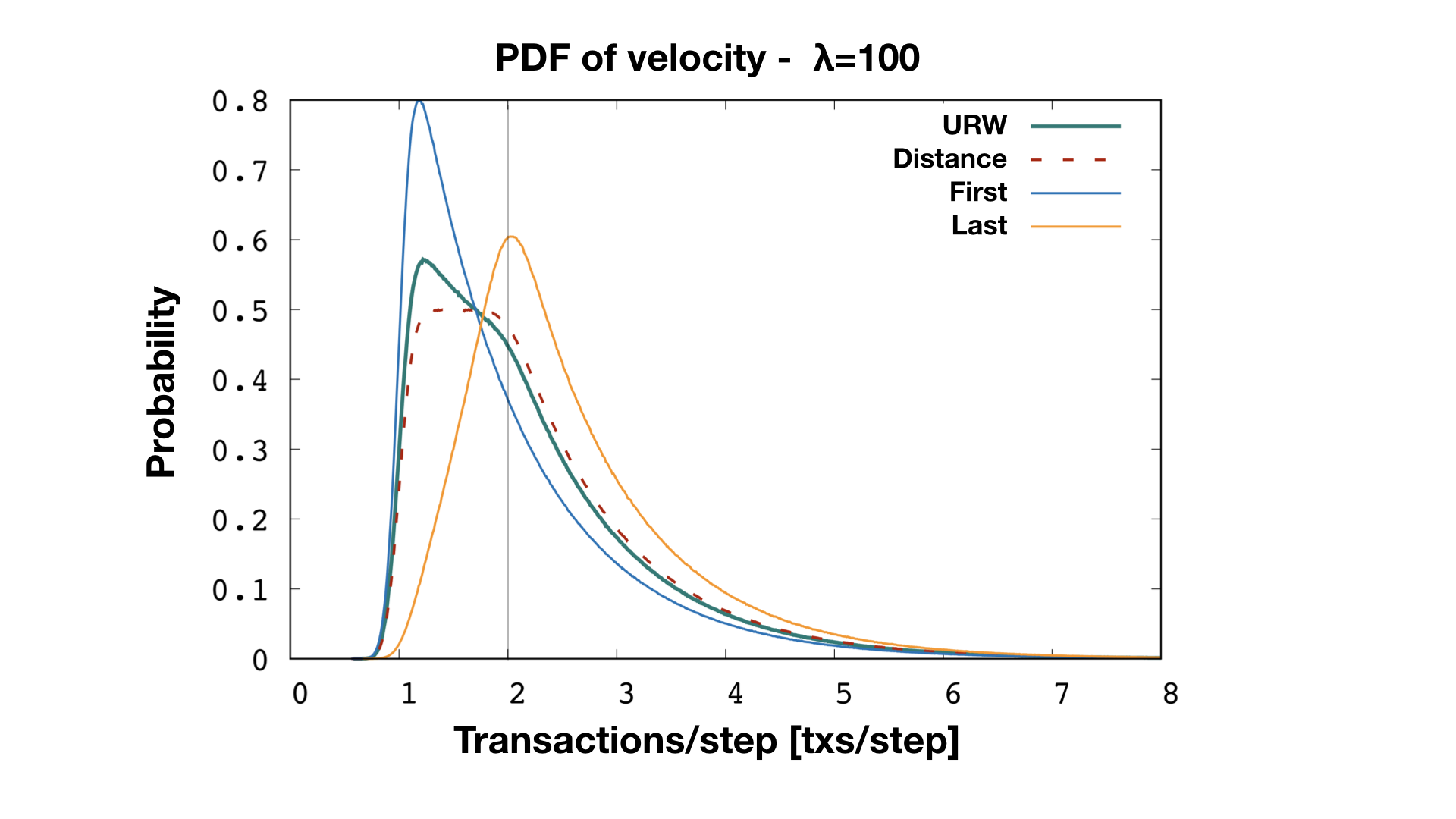
Here, we show the PDF of the velocity. Data points have been normalized to units of transactions (i.e., divided by λ). Blue and orange lines are velocities measured when random walkers always advance to the first approver and the last approver respectively. These curves are important because they give us lower and upper bound on velocities. The green curve is the velocity of a URW, and it is the one answering our previous question. Last but not least, the red dotted line is the distance between each transaction and its direct approvers. It gives us information on the structure of the Tangle. More specifically, it shows the probability distribution of how long the links connecting two transactions are.

We have seen what the velocity of random walkers is in the case of an unbiased walk, corresponding to α=0. Now, we can have a look at the average velocities of biased random walkers for different values of α. For this experiment, we consider several Tangles, each one built with different values of both α and the incoming transaction rate λ. We then measure average distance and velocity.

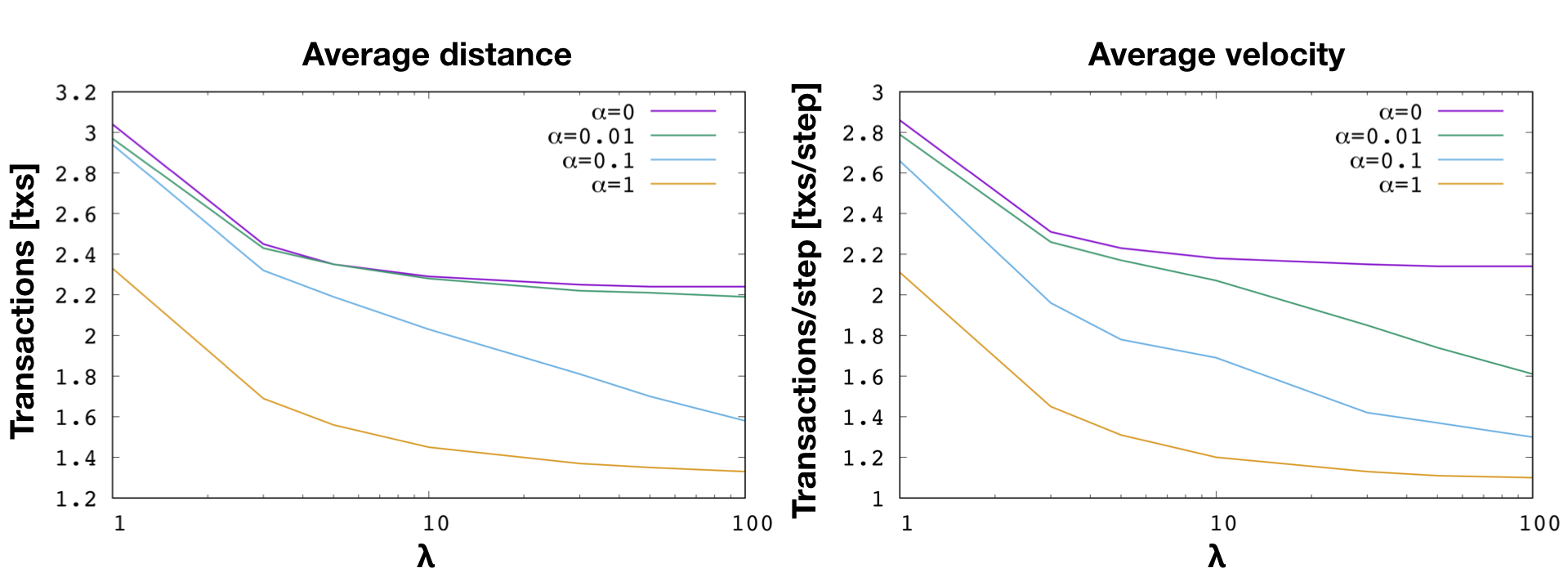
Here, we can see the average distance (on the left) and velocity (on the right) as a function of λ. The plots show x-axis in logarithmic scale. The average of both distance and velocity decreases when increasing α and λ values. This result depends on the impact that both α and λ have on the structure of the Tangle. The bigger the parameter α, the more likely random walkers are to transition to transactions with higher cumulative weight. Moreover, as discussed in our blog post on direct approvers, a change of α results in a change in the number of direct approvers, thus suggesting a higher probability of having links within a shorter distance. Similarly, by increasing λ, more transactions are announced within the same time unit h, resulting in a higher probability of creating links with shorter distances.

Knowing how long and how fast (or slow) our random walkers run can be very useful when doing analytical approximations of the parasite chain attack. It is also useful when slicing the Tangle into groups of consecutive transactions so that each random walker passes through approximately one transaction from each slice. Moreover, it can help to better understand how the computational effort of performing random walks is spread.

Our research team is currently studying this topic. In particular, we are interested in looking into the following questions:

Can we find an analytical formula that describes the PDF of the velocity?
How does the velocity change if random walkers walk in a backward direction (i.e., from present to past)? This could be useful, for example, when considering the case of random walkers stepping back if a transaction doesn’t fulfill a given condition.
Is there a relation between the probability of a tip being left behind (i.e., becoming a permanent tip) and the velocity?

We will work on these questions as well as on the relation between velocity and the parasite chain attack. In the meantime, you are all very welcome to ask questions and discuss this topic here or in our Discord channel #tanglemath.